How To Create A Search Bar In Google Sheets? – 3 Simple Steps To Follow

Google Sheets is a free online spreadsheet application that allows you to create spreadsheets that can be shared with others. It’s a great tool for organizing data and sharing it with other people. One of the best things about Google Sheets is that you can easily add features to your spreadsheet by using formulas and functions. In this article, we’ll show you how to create a search bar in Google Sheets in 3 simple steps.

How To Create A Search Bar Or Search Box In Google Sheets?

To create a search bar or search box in Google Sheets, you can use the Conditional Formatting combined with =SEARCH() formula.

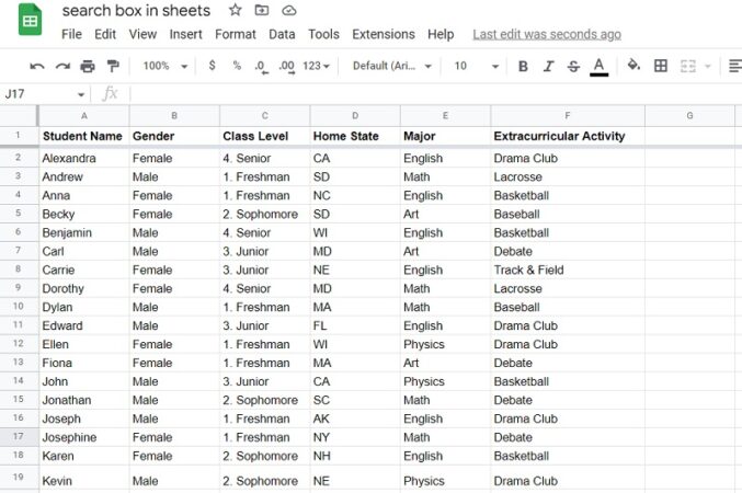
Let’s see the example data sheet I used in this post. In the student list below, I want to search the Class Level. So, here are steps on how I create a search bar for this purpose.

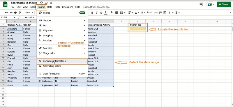
Step 1. To create a search box, you need to name the selected cell used for searching first. Remember that this “box” needs to be outside the data range. Here, I selected the cell H2 as my search bar. Then, you select the data range you want to search, which is A2:F19 in my example. Then, go to Format –> choose Conditional formatting.

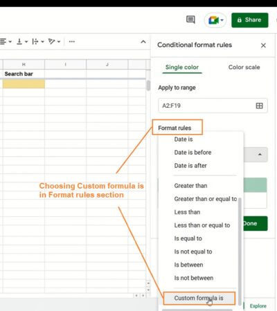
Step 2. On the left side, the Conditional format rules panel appears –> subsequently choosing Add another rule. In the section Format rules, choose Custom formula is in the drop-down list.

Step 3. In the Value of formula box, you need to input the SEARCH formula. The formula in my example will be: =SEARCH($H$2,$C2)>0. After that, click Done, and type the text you want to search for the Class Level in the cell H2, or the created search bar. Let’s see the result below.

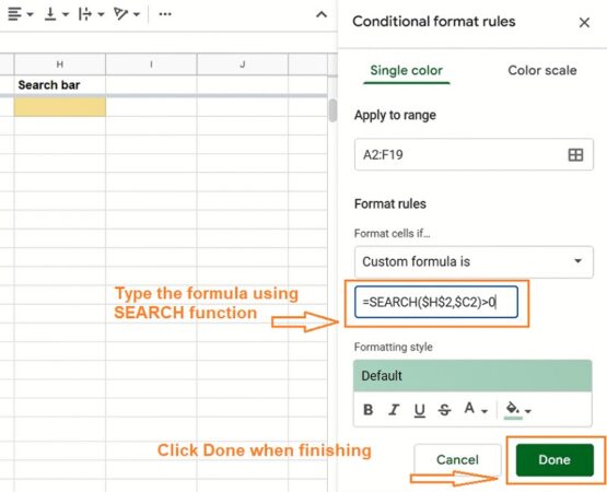
I will demonstrate how we can form the above formula using the SEARCH function.

• Initially, we type =SEARCH( to let the sheet know we want to input a formula. The box will have a red border in this step because the formula is not finished, so don’t worry.
• Then, we need to fix the cell for the search bar, no matter what happens, so we use the dollar symbol $ in front of the column letter and the row number, as $H$2.
• After that, we need to fix the column for the search range but not the row because we want the highlight to shift as the text in the search box H2 changes. So, we use the $ symbol before the column letter like $C2. Now we’ve done the SEARCH function, so we use a closing round bracket to finish the formula.
• We add >0 after the SEARCH function because we want it to highlight the row if the SEARCH function returns a number (the SEARCH has values). That’s why we have the formula =SEARCH($H$2,$C2)>0.

Here is the result after we complete all steps:

FAQs

Video: Create A Search Bar In Google Sheets Step By Step

Share on Facebook

Tweet

Follow us

Save

Andrew N. Keegan

Andrew N. Keegan is a self-proclaimed “tech junkie” who loves consumer electronics. He loves Apple products and is always in line for the newest iPad. In addition, he loves technology, Office products, and social media.

He was continually attempting to figure out his family’s computer. This thing led to an interest in how technology may improve our lives. He holds a degree in IT from NYIT and has worked in IT for over a decade. Since then, he’s been hunting for new goods to share with friends and family.

Andrew N. Keegan loves video games, tech news, and his two cats. He’s also active on social media and shares his latest tech finds.